Making The Raspberry Pi Blink

a computer human at a rave

In the last post, we covered ELFs and memory layouts. I concluded the article with the promise of walking through an example program in execution to help visualize things better.

a gif of a muppet that reads "I lied"

I’m sorry but this new stuff seemed more appealing 😔. We could probably follow it up in a separate post but for now, let’s jump straight to the Raspberry Pi!

Plugging it in

an image of a raspberry pi that has a red blinking light

Nothing happened. Why? For starters, we have no output devices for the Raspberry Pi to convey any information to us. And more importantly, we don’t have any software on this Raspberry Pi that could put our output devices to use.

Computers come with very little pre-packaged code; stuff like performing basic checks to ensure the hardware is functional. But apart from that, it has just enough code to load your operating system. The operating system then takes care of everything else.

For Raspberry Pi, I think the sequence of operations looks something like this

  1. Perform hardware checks
  2. Load the operating system from the SD card with a file named kernel8.img.

Let’s start with the operating system for our Raspberry Pi; Raspbian; an operating system built by the company manufacturing Raspberry Pis. I’ve downloaded this onto an SD card. This is what the contents look like.

an image of the contents of the sd card

My guess is as good as yours on what these files are. But I do recognize the kernel8.img file on the SD card. That is the ELF executable of the operating system that is run when the Raspberry Pi is booted. In other words, it’s the “.exe file” of our operating system. (It uses an ELF file type because Raspbian is built on top of Linux).

If I boot the Raspberry Pi with the SD card plugged in, the logo pops up on the display alongside a welcome message.

an image of raspberry pi writing to a connected lcd display

Your operating system converted the hardware you had into a fully functioning computer ready to be used. So how does the operating system do this? What does the code interacting with hardware look like?

Write your own OS

I need to start this section with a disclaimer. I have next to no practical experience working with hardware. A whole lot of this is new to me; best practices are not expected to be followed and mistakes are expected to be made ^_^.

With that, let’s get started. In our previous post, we’ve seen what ELF files are, and how they are combined to form an executable file. We’ll also start using C rather than writing this in assembly. I mean… I’m bored, but I’m not that bored.

Let’s start with a bare minimal operating system that does nothing.

void main() {
    while(1);  // Loop infinitely; do nothing
}

(Note: Programs start execution at the main function by default). Let’s build this into an ELF file, load it into our SD card, and see what happens.

the same raspberry pi with nothing on the connected lcd screen

Aaaand lights out. Obviously, our operating system right now does nothing. It might not look like much but right now, our CPU is working pretty hard on that infinite loop. However, some proof of life would be nice. We could start writing code that prints “Hello World!” onto the screen. That would be a great way to verify that our operating system is working as expected. However, writing to a display isn’t as straightforward as we’d imagine. We’ll get to it in a future post but for now, let’s start small.

Making an LED Blink

Taking a look at the Raspberry Pi model again, we see the 40-Pin General-Purpose Input/Output GPIO. We’re going to control these pins to make our Raspberry Pi do something useful.

an image of the model of the raspberry pi

Let’s take a closer look at the layout for these pins (found this in the documentation).

an image of the raspberry pi pin layouts from pin 1 to 40 with markings of what the pin does

Each of these pins has a base function. For example, Pin 1 is marked as 3V3 power. This means that Pin 1 is at a +3.3 Voltage. Similarly, Pin 6 is marked Ground or 0V. So if I connect an LED bulb marked for 3.3V across Pin 1 and 6, I should expect it to glow.

a raspberry pi with a bulb connected that is currently glowing

Some pins are also labelled with a GPIO number, like Pin 3 marked as GPIO 2. These pins are of interest. The pins marked GPIO can be programmatically controlled. For example, your code could set the pin to output 3.3V (HIGH) or ground the pin to 0V (LOW). So if I connected the same LED across Pin 3 (GPIO 2) and Pin 6 (Ground) and alternated Pin 3 between 3.3V and 0V with a pause between each switch, I’d make the LED blink!

Then, the last piece of the puzzle would be, how do we control Pin 3 (GPIO 2) with code. For this, we’ll need a quick detour to explain Memory Mapped IO.

Memory Mapped IO

As covered in an earlier post, your RAM has memory addresses which refer to the memory locations in your RAM. They’re almost like coordinates on your RAM. Your CPU reads/writes to your RAM via memory addresses; “store the number 50 at address 0x80000000 (hexadecimal)” or “read the value present at address 0x125AF724”. However, your CPU also reserves some addresses that don’t really correspond to any location in the RAM. Instead, these addresses map to your IO devices. When you read/write to these addresses, your CPU knows you’re trying to access hardware and takes care of interacting with the hardware. For example, your CPU documentation could specify that, on writing the number 1 to address 0x70000000, it sets the GPIO 2 pin to 3.3V.

This model of virtualizing the hardware with memory addresses is referred to as memory-mapped IO. It makes it awfully convenient to write code. You write to these memory addresses as you would for reading/writing data to RAM and your CPU takes care of the rest.

Manipulating the pin

At this point, we’re ready to manipulate the pin to make our LED blink. Let’s refer to the documentation on the memory address of the GPIO Pins. Taking a look at the BCM2711 peripherals documentation (the CPU used on our Raspberry PI), we see several registers along with their memory address and function, we’ll need several registers but let’s just focus on one for now.

a snippet of the documentation of each register in raspberry pi

The documentation further explains what GPSET0 does here.

a description of what gpset0 register does. covered in the following lines

tldr; to set the GPIO Pin n to a high (3.3V) voltage, we have to set the nth bit of this memory address to a 1. So in our case, setting this memory address to binary 00000000 00000000 00000000 00000100 (2 in decimal) would set GPIO Pin 2 to High. There’s a similar memory address GPCLR0 for which setting the same value would clear GPIO Pin 2. Let’s see what the code looks like.

enum {
    BASE = 0xfe200000,  // Base address of the registers according to the docs
    GPFSEL0 = BASE + 0x00,  // Offset from the base (refer to register view image)
    GPSET0 = BASE + 0x1c,
    GPCLR0 = BASE + 0x28,
};

volatile unsigned int *register_gpfsel0 = (volatile unsigned int*) GPFSEL0;
volatile unsigned int *register_gpset0  = (volatile unsigned int*) GPSET0;
volatile unsigned int *register_gpclr0  = (volatile unsigned int*) GPCLR0;

void clear_pin(int pin_number) {
    *register_gpclr0 |= 1 << pin_number;
}

void set_pin_as_output(int pin_number) {
    *register_gpfsel0 |= 1 << (3 * pin_number);
}

void set_high(int pin_number) {
    *register_gpset0 |=  1 << pin_number;
}

void spin_wait(unsigned long n) {
    for (unsigned long i = 0; i < n; i++);
}

void sleep() {
    spin_wait(1000000);
}


void blink_led() {
    set_high(2);
    sleep();
    clear_pin(2);
    sleep();
}


void main()
{
    set_pin_as_output(2);
    while (1) {
        blink_led();
    }
}

Code Walkthrough

There’s quite a lot going on here. Let’s break it up into pieces to better understand.

enum {
    BASE = 0xfe200000,  // Base address of the registers according to the docs
    GPFSEL0 = BASE + 0x00,  // Offset from the base (refer to register view image)
    GPSET0 = BASE + 0x1c,
    GPCLR0 = BASE + 0x28,
};

volatile unsigned int *register_gpfsel0 = (volatile unsigned int*) GPFSEL0;
volatile unsigned int *register_gpset0  = (volatile unsigned int*) GPSET0;
volatile unsigned int *register_gpclr0  = (volatile unsigned int*) GPCLR0;

We start by creating three variables register_gpfsel0, register_gpset0 and register_gpclr0 that point to the memory addresses specified by GPCLR0, GPSET0 and GPCLR0 respectively. These are the addresses that we found in the documentation. Essentially, we’ve created handy variables to read/write to these memory-mapped addresses.

void set_high(int pin_number) {
    *register_gpset0 |=  1 << pin_number;
}

We then created several functions that abstract away the registers and make it more intuitive to use these addresses. The set_high , for example, sets the right bit for a given pin_number to a 1. We do this based on the documentation specified for the GPSET0 register. For example, calling the functionset_high(2) sets the bit associated with GPIO 2 to a 1, consequently setting GPIO 2 to a high voltage.

void blink_led() {
    set_high(2);
    sleep();
    clear_pin(2);
    sleep();
}


void main()
{
    set_pin_as_output(2);
    while (1) {
        blink_led();  // call blink_led function in an infite loop
    }
}

Putting it all together, our new main function initializes GPIO 2 and goes into an infinite loop that calls the blink_led function. What does this function do? It first sets GPIO 2 to a HIGH, proceeds to sleep for a fixed duration, clears GPIO 2 and goes straight back to sleep.

Repeat this an infinite amount of times and you should get a blinking LED light. Let’s build this and plug our new operating system into the Raspberry Pi.

a gif of the raspberry pi and the led blinking

Success! Proof of life for our “operating system”!

Wrapping it up

At this point, we’ve successfully manipulated some hardware with code even if it’s just to blink an LED bulb. However, that’s pretty much all our operating system supports. It’d be cool if our operating system could do a little more than what it is currently capable of. But for now, we’ve covered enough to call it a day.

Running Assembly Code

an assembly line of computers assembling stuff

In the previous post, we established some (very) high-level context in place about what we need to get our code to run on a computer.

A quick recap:

  1. Need a working CPU that can access a working RAM
  2. Need instructions for the CPU in a language it understands (assembly code native to its instruction set).

We’re nowhere close to having sufficient context to see the big picture yet but we might be ready to start seeing some of the basics in action. Let’s start by running some assembly code.

Hello World!

Note: I write most of this code on my x86 Linux system. Although I've tried to omit irrelevant details / cut corners / outright lie, parts of this section can be understandably confusing. If you're having trouble visualizing any of this, stick around until we go through an example. Hopefully, that should help you visualize all of this a little better.

Just as you have your executable “.exe” files in Windows which actually runs a program on double click, Linux has a binary format called ELF (Executable and Linkable Format). The ELF format is just a binary standard on what a program “should look like”. Think of it as a recipe in a very specific format. This recipe gives Linux all the information it needs to start a process (a running program).

So it goes something like this: When you run an executable ELF file, Linux starts an “empty” process (the process has been allocated resources such as memory) and asks a program called the loader to load your ELF into this process. So your ELF has the logic and the process Linux gave you has the resources your logic can make use of. Here’s an actual footage of the process in action (or at least how I visualize it).

ELF Sections

Let’s try to understand the ELF format a little better. The ELF file is broken down into several sections. Each stores one category of data. Let’s take a look at some of the sections that are relevant to us

  1. .text – This section contains the code for your program
  2. .data – This section contains stuff like global variables, any pre-set variables, etc.
  3. .bss – This section contains stuff like unset variables
  4. .symtab – This section contains a table that maps all the symbols you’ve used. You might have used fancy variable/function names in your code but your computer doesn’t understand these symbols like you do and thus stores it in a table for easy access.

Process Memory

While we’re at it, it would also do us some good to better understand how memory is laid out for a process. To recap, Linux first creates an “empty” process for the ELF file to be loaded into. This process is also assigned memory that your code can make use of. The memory layout of a process can be visualized in a format like this (you could think of this as each process in Linux getting a special suitcase with all these compartments to store all of its data)

As you might have already guessed .text portion of your ELF file goes to the TEXT part of memory. The .data portion of your ELF goes to Initialized Global Data. The .bss part of your ELF goes to the Uninitialized Global Data BSS part of memory.

The majority of the memory your process has access to however, is split between Stack and Heap. Think of them as analogous to your Checking and Savings accounts. Your Checking account helps you meet your day-to-day expenditures. You use it frequently but the value of individual transactions made on your checking account is likely to be small. Our stack is like our checking account.

The heap, on the other hand, is like your Savings account. You use this less frequently compared to your Checking account but you’re probably only using it to move larger amounts of money.

Time to get our hands dirty!

We’re ready for some code now! This is what the first part of my Hello World program looks like. It defines what it wants printed, sets the stage for the print function (the second part of the code) and hands control over to it.

.data  # Begins our .data section
    msg:  # Create a symbol called "msg"
        .asciz "Hello World!\n"  # with type asciz (string) and value "Hello World!\n"

.text # Begin our .text section
.extern print # Call out there's a function named "print" that is externally defined
.globl main # Make the symbol "main" globally available

main:  # Define the symbol "main". All the lines till #18 belong to main
    push $14  # Add number 14 to the stack which is the number of characters in "msg"
    push $msg # Add the address of msg to the stack
    call print # Call the print function 

    movl $1, %eax # Lines #14 to Lines #16 are to correctly exit the program
    movl $0, %ebx
    int $0x80
hello.s

So the idea is this, we can ask an assembler to generate an ELF file for this piece of code. We define the .data section of our ELF file from Lines #1 to #3 where we define a string variable named msg with the contents “Hello World!\n”.

Lines #5 to #16 is the .text section of our ELF file that contains the actual code. There’s actually quite a bit going on here and is understandably confusing. But the important parts of this code are from Lines #10 to #12 where we set the stage by writing the inputs our print function requires (the string to print and the number of bytes in the string) to the stack part of the memory (with the push command) and call the print function.

We can generate the ELF file out of our assembly code by running the assembler. We can also read the ELF file with the objdump utility in Linux.

as hello.s -o hello.o  # Generates our ELF file named hello.o

file hello.o  # Use the file utility to see the type of hello.o generated
hello.o: ELF 64-bit LSB relocatable, x86-64, version 1 (SYSV), not stripped

objdump -d hello.o   # Decode the .text section of our ELF file
hello.o:     file format elf64-x86-64


Disassembly of section .text:

0000000000000000 <main>:
   0:	6a 0e                	pushq  $0xe
   2:	68 00 00 00 00       	pushq  $0x0
   7:	e8 00 00 00 00       	callq  c <main+0xc>
   c:	5b                   	pop    %rbx
   d:	b8 01 00 00 00       	mov    $0x1,%eax
  12:	bb 00 00 00 00       	mov    $0x0,%ebx
  17:	cd 80                	int    $0x80

objdump -s -j .data hello.o  # Decode the .data section of our ELF file
hello.o:     file format elf64-x86-64

Contents of section .data:
 0000 48656c6c 6f20576f 726c6421 0a00      Hello World!..  

The decoded .text section of the ELF file does infact have the code wrote and the .data section shows the Hello World! string as expected. So far so good!

The other half of our assembly

As of now, we have an ELF file but it’s not quite ready to be run. Why? For starters, we’re missing the print function we call on Line #12. The only reason we were able to generate an ELF file out of this assembly code despite missing a function is that we promised the ELF file that the definition for a “print” function would come from an external source (from Line #6). So let’s create a similar assembly file that defines our print function (note, this function is terribly oversimplified to a point it’s almost wrong to be using it. But it should suffice for our example)

Let’s call this code print.s with the following definition

.text
.globl print

print:
    mov $1, %rax
    mov $1, %rdi
    mov 8(%rsp), %rsi
    mov 16(%rsp), %rdx
    syscall
    ret
print.s

All this really does is, it reads inputs from the stack and asks our operating system to print out that string. We once again generate an ELF file for this code.

At this point, we have two ELF files in our hands (one named hello.o that was generated from hello.s and the other print.o generated from print.s). We’re ready to combine the two ELF files into one that we could actually run.

Linking

The software to combine multiple ELF files into one is done by a software unsurprisingly referred to as the Linker. Each ELF file has its own sections (like the .text, .data and so on) and we need someone to combine corresponding sections into one. For example, the .text section of each ELF file needs to combined into a single one (and similarly for other sections). The linker also does this nifty thing called relocation but let’s not get into that right now.

This is how we’d go about linking our ELF files into one named runELF

ld -e main hello.o print.o -o runELF    # Combine hello.o and print.o to generate runELF
./runELF  # Executing the runELF file prints out Hello World! 
Hello World!
ShellScript

While we’re at it, we should probably try to disect he generated runELF file to verify the things we’ve seen so far.

file runELF  # See what type of a file runELF is
runELF: ELF 64-bit LSB executable, x86-64, version 1 (SYSV), statically linked, not stripped

objdump -d runELF  # Print the .text section of runELF

runELF:     file format elf64-x86-64


Disassembly of section .text:

0000000000401000 <main>:
  401000:	6a 0e                	pushq  $0xe
  401002:	68 00 20 40 00       	pushq  $0x402000
  401007:	e8 0d 00 00 00       	callq  401019 <print>
  40100c:	5b                   	pop    %rbx
  40100d:	b8 01 00 00 00       	mov    $0x1,%eax
  401012:	bb 00 00 00 00       	mov    $0x0,%ebx
  401017:	cd 80                	int    $0x80

0000000000401019 <print>:
  401019:	48 c7 c0 01 00 00 00 	mov    $0x1,%rax
  401020:	48 c7 c7 01 00 00 00 	mov    $0x1,%rdi
  401027:	48 8b 74 24 08       	mov    0x8(%rsp),%rsi
  40102c:	48 8b 54 24 10       	mov    0x10(%rsp),%rdx
  401031:	0f 05                	syscall 
  401033:	c3                   	retq  
  
objdump -s -j .data runELF 

runELF:     file format elf64-x86-64

Contents of section .data:
 402000 48656c6c 6f20576f 726c6421 0a00      Hello World!..  
ShellScript

Relocation

Unsurprisingly, the .text section in runELF is a combination of the .text section of hello.o and print.o. So, all the instructions in the .text of hello.o should be contained in the .text section of runELF (which is what we do see here). However, they’re not exactly identical. Let’s pick a line from hello.o and pick the matching line from runELF and compare them.

 d:	b8 01 00 00 00       	mov    $0x1,%eax        # Line 17 in the .text of hello.o
   vs
 40100d:	b8 01 00 00 00       	mov    $0x1,%eax  # Line 16 in .text of runELF
ShellScript

As you can see, the instructions are identical mov $0x1,%eax vs mov $0x1,%eax (b8 01 00 00 00 is just a hexadecimal representation of mov $0x1,%eax). The difference however is the characters that come before the colon. In .text section of hello.o, this character is “d” whereas in runELF, it’s “40100d”. These characters are hexadecimal numbers and they reference the location in memory where this instruction can be found when running the ELF. This is what we mean by “relocation”. The linker has essentially combined the two ELF files and assigned each piece of data a location in memory.

Relocation isn’t expected to be making much sense at the moment. Perhaps seeing an example of this ELF file loaded into memory and in a running might help.

Wrapping Up

At this point in time, I’m fighting the urge to keep going on with some analysis of the actual execution of the code. But this seems like a logical place to stop.

A quick recap of what we’ve seen first. We’ve so far dissected ELF files without things getting too ugly (I hope?). At the same time, we’ve also taken a VERY quick look at the memory layout of a process. I don’t expect this part to make sense yet as we haven’t really gone through an example.

In the next post, let’s walkthrough the execution of runELF step by step.

Running Code – Overview

a cartoon of a computer finishing a marathon

This is the first part of a series of posts in an attempt to piece together how your computer really runs your code. The topic by itself could have an entire book dedicated to it, but I’m going to see if we can cover the essentials without delving too much into the nitty-gritty details (after all, these posts are intended to be beginner friendly). A quick note before we get started, I am by no means an authority on the subject. If something seems inaccurate, please do let me know.

A quick recap on computers

Every computer comes with a series of hardware components. Let’s take a look at a Raspberry Pi 4 – a miniature computer.

a raspberry pi model

There’s quite a bit going on in this image, but what we’re interested in at the moment is the Broadcom BCM2711 CPU and the 8 GB RAM chips. Two of my previous posts briefly cover the workings of both of these (CPU, RAM). (There was supposed to be a part 2 for some of these topics but well… life is short and so is my attention span).

RAM

In a nutshell, the RAM can be visualized as a linear sequence of bytes that can be read or written to. Each byte in the RAM has a reference number we call “address”.

a visualization of ram as an array

For example, the memory address 0x0000 (in hexadecimal) stores 1 byte (8 bits) of information 00000000. If you wanted to read the 285th byte in your RAM, you would want to access the memory location 0x011d (285 in the decimal system).

CPU

The CPU supports several basic operations your code could use which are defined by the manufacturer of the chip. This chip supports the ARM instruction set. The instruction set of a chip supports a fixed set of predefined operations such as ADD; which adds two numbers, or the LD/ST; which loads / stores data to a memory location (the full list of operations supported can be found online).

Your CPU doesn’t deal with individual bytes. A single byte is nowhere close to being large enough to store anything meaningful. Therefore, your CPU defines a “word”, which is the number of bytes that it typically works with at a time. This is what we mean by a “64-bit” computer. Your computer defines the word size to be “64 bits”. Or that is, it’s capable of working with 64 bits / 8 bytes of data at a time.

Apart from the memory in the RAM, a CPU comes with registers that are extremely high-speed memory locations that the CPU can use. Think of registers as the CPU (core)’s personal fanny pack while the RAM as a suitcase that it shares with the other cores. All the stuff that a core requires at any given moment is typically stored in the fanny pack. It’s easy to access but has limited storage.

A CPU comes with anywhere from 16 – 30 registers that it can use and each register is the size of the word, 64 bits for a 64-bit CPU. How are these registers used? Say you ask your computer to add two numbers, your CPU loads the two numbers from the RAM into registers, runs the ADD operation on the two registers, and stores the result back into the RAM (not always the case but it’s typical).

All of this should be a lot clearer when we see some examples in action. For now, all I want you to remember is the following:

  1. A CPU (core) comes with a set of registers which are high speed memory locations for the CPU to read and write to. A CPU also has access to the RAM.
  2. Any operations your CPU performs, has to either be performed on a register or in the RAM. If you want your code to modify a text file, it (or at least the part of it that you need to work with) needs to be loaded first into the RAM.

The End Goal

So, where are we going with all this? Essentially, whatever code you intend to run, needs to first be converted into something your CPU understands. What this means, is that each instruction in your Python / Java / C++ code needs to be translated into one or more instructions defined in the instruction set of your CPU.

There are several different approaches to go about this translation each of which have their own pros and cons.

Compilers

Languages like C / C++ take this route. Compilers convert your code into a low level language compatible with your computer’s instruction set. We call this converted code, assembly code. So each time you want to run your code, you “run” the assembly translation of your code. The translation to your assembly code is a one-time process (unless of course, you make changes to your code, you need to retranslate).

The advantage of this approach is that the compiler has translated your code into something that is native to your computer. So your computer has a fairly easy time when actually running your code.

But what happens if you want to run your code in a different system that runs a different architecture? The assembly code you generated was native to your computer and there’s a chance it might not work on my computer (if my computer runs a different operating system or has a different instruction set). Therefore, to run your code, I would need a separate compiler that knows how to translate your code to something my computer understands.

The Bytecode Approach

The downside in the previous approach was that the assembly we converted our code to was machine dependent. And the bytecode approach addresses just that. Here, we translate code to something that looks like the assembly we would have seen in the first approach except that this assembly is machine independent; which we call bytecode. Your code did get translated to something low level but it’s not something our computer understands (since after all, the only thing your computer can run is something its instruction set can understand). So… how do we run this on our computer…?

a meme that reads "that's the neat part. you don't"

To actually run this bytecode, you need to have a separate piece of software running in your computer that is specialized at running your bytecode. We call this a “virtual machine” as this software mimics a computer whose instruction set is the same as that in your bytecode. This is a separate topic by itself so we’ll stop here for now. The key takeaway is that the advantage of bytecode is that it is independent of your computer hardware. The same bytecode that was built on your computer can be run on a different computer (as long as this different computer has a virtual machine installed that is able to run this bytecode).

Java typically takes this route.

Interpreters

This is the lazy way out (not necessarily a bad thing). The interpreter reads a line of your high level code, figures out how to translate this to something your computer can understand and runs this line before moving on to the next line. Notice how unlike the previous approaches, the interpreter translates AND runs your code in the same pass. In the previous approaches, you had your code translated to an intermediate low-level code (assembly / bytecode). Each time you want to run your code, you just need to run the low-level code directly as the translation has already been done. There is no need for retranslation each time you want to run your code.

Whereas in an interpreter, each time you want to run your code, the translation phase is redone.

This makes interpreted implementations of a language slower but it gives some added flexibility which we can explore in a separate post.

Wrapping it up

So far, we’ve covered the need to translate your code to something your computer can run and three approaches that are typically taken to get there.

Most questions however still remain unanswered. How does a compiler translate your code to something my computer understands? How does your code interact with various devices that your computer comes with (such as your monitor or WiFi) to make something useful happen? What does this assembly code actually look like and how does it actually run in your computer?

We’re still missing a quite a bit of context but I think we should be ready to see some basic examples. In the next post, we’ll see some of this in action on a 64 bit AMD computer that runs Linux.

The Coding Interview And How Best To Prepare

coding interview depiction

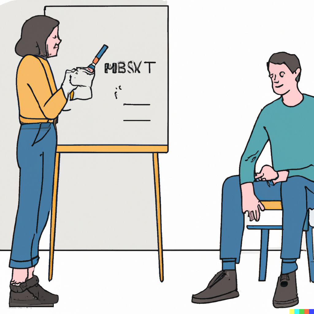
In the previous post, we saw a general outline of the interview process and a few pointers on how to polish your resume to help you stand out. In this post, we’ll cover a little about the coding interview.

The kind of interview you need to prepare for largely depends on the level and the type of position you apply for. Thus, it’s important that you clarify the kind of interview you can expect with your recruiter ahead of time.

For example, if you’re applying for the position of Senior Backend Engineer, you’re more likely to have a design-focused interview. However, if you’re relatively new to the industry, your interviews will tend to be based on your understanding of Data Structures and Algorithms.

a pencil sketch of a coding interview

The Coding Interview

If I’m being honest, I have no love for the coding interview. However, I do understand (kinda?) why these interviews have become the de facto process for hiring in tech. Ideally, firms would love to hire everybody as an intern and use performance during the internship as the sole basis for hiring. This system works a lot better for everyone involved and is definitely a more accurate measure of a candidate’s skill.

However, this process is simply impractical at scale and that is what leads us to this situation we find ourselves in.

The coding interview is typically a 45-50 minute long interview where your interviewer provides a problem statement. You are then expected to solve this problem in code as efficiently as possible making use of appropriate data structures and algorithms.

How best to prepare for your coding interview

A quick disclaimer before we get started. Most of this isn’t new information. The intent of this post isn’t to try and peddle some kind of a “secret” to cracking the coding interview. Instead, it will be to re-emphasise a tried-and-tested set of resources which I can personally vouch for.

To start us off, I’d recommend a book; Cracking The Coding Interview by Gayle Laakmann McDowell. The book is an absolute classic and will get you started on Algorithms and Data Structures. There are some great tips and insights about the interviewing process itself in addition to the technical aspect which I will best leave to the author. Make sure you’ve done all the exercises in the book before moving on.

However, I do believe that the book by itself isn’t sufficient for some of the tougher interviews out there. Leetcode is highly recommended to reinforce what you’ve learnt from the book.

The Leetcode Grind

Leetcode is definitely the gold standard platform for interview preparation and there’s a high chance that your recruiter will recommend it to you themselves. I’d suggest solving the following in order

  1. Leetcode – Top 100 Liked Questions
  2. Leetcode – Top Interview Questions (there should be a significant overlap between the two)

If you’ve never done any sort of competitive programming prior to this, this might be an unpleasant journey at the start but I promise it gets better over time. Start off with the ones marked Easy. When you start getting comfortable with Easy, move on to Medium and so on.

Spend no more than 30 minutes per question. It feels amazing when you’re immediately able to solve a problem. But the questions that you don’t have an immediate solution to are the ones that help you identify gaps.

If you aren’t able to come up with a solution for a question in time, look at the solution in the Discuss tab and understand the solution. But make sure to perform some kind of retrospection on why you weren’t able to come up with a solution. Did you spend too much time in one line of thought? Maybe the key to solving the problem was using some key information that you missed in the question. If so, why do you think you missed this hint? This does two things for you; it helps you avoid making a similar mistake in the future and more importantly, it forces you into the habit of thinking in new ways for any problem you attempt in the future. Maintain some sort of notes so that you also have something to look back to.

Structure your thought process

Interviewer: *provides problem statement*

Candidate: “Okay I think sorting this and performing a binary search should work”

Interviewer: *provides a scenario where it wouldn’t work*

Candidate: “Okay then I think converting this to a tree and performing a Depth-First-Search should work”

Interviewer: *provides a scenario where this wouldn’t work*

This approach has next to no structure. In my opinion, having a good structure in the way you approach a problem is the single greatest quality in a candidate. You can think of it this way; all the algorithms you’re able to implement are tools in your toolbox. So it’s great if you have a well-stocked toolbox but it’s not what anyone’s looking for. I’d rather pick the candidate that can build a whole bridge with just a hammer (this is also why everybody loves the villagers in Age of Empires 🙃).

A structured thought process lets you look past all the noise in a problem, reduces the problem to its core and can suggest various approaches to solve this reduced version of a problem. While you solve Leetcode Medium and Hard problems, try to deliberate with this. Even if you think you can solve a problem immediately, try to apply some sort of structure on why your solution might work.

“How many Leetcode problems should I solve?”

I have no idea how to answer this question. Some folks are regular on platforms such as Codeforces whereas some are not. Some might have taken a course on data structures and algorithms at some point whereas some may have not. So how much practice you need depends entirely on your background. All I can tell you is, on average, you should be able to solve a Leetcode Medium problem and have a 20-30% chance of solving a Hard problem. That number is just my personal opinion on how prepared a candidate should expect to be for a hard interview.

Write code on paper?

Your objective is to write clean code in one pass. No back and forths of any kind, no spamming the Run button to see if your code compiles etc. That is, you write code once and it does exactly what you intended to do and it passes all test cases. All in one go. It’s no easy task to get to this place but you should be able to do it with sufficient practice.

For this reason, I recommend that once you have sufficient practice on Leetcode you should also practice writing code on paper / Google Docs / Notepad. In your actual interview, you might be expected to write code on a whiteboard or on a platform that doesn’t provide any sort of syntax highlighting so some practice might make you a little bit more comfortable during whiteboarding. This practice also forces you to think through everything ahead of time since it’s a lot harder to perform corrections when writing code with pen and paper.

Mock Interviews

Honestly, do yourself a favour and find someone to conduct a few mock interviews for you. Preferably someone from the industry that has experience conducting SWE interviews. So far, you’ve been practising solving problems by yourself and have put next to no effort into presenting your work to someone else. This is a great way to allow confirmation biases to creep in. Getting someone else to help identify potential flaws in the way you present your work is definitely going to be worth your while.

The Interview

His palms are sweaty, knees weak, arms are heavy
There’s vomit on his sweater already, mom’s spaghetti

It’s time for the interview! It’s not easy to stay calm during your interviews (I know I wasn’t 🥲). But you’ve got this! In this section, I want to talk a little about some things to watch out for during your actual interview.

Think out loud!

Your interviewers are usually instructed to nudge you in the right direction if you seem stuck. It happens way too often that candidates sit in absolute silence whilst thinking to themselves, sketching something on the whiteboard every now and then. It can be pretty confusing for your interviewer to gauge if you’re in need of help.

Therefore, think out loud! Talk about various approaches that you think can and cannot work. I cannot emphasise this enough. Your interviewer isn’t there to see if you’re able to solve a problem or not. They’re there to gauge how you approach a problem.

Making assumptions

Sometimes, you might wish there was a utility method that does something trivial that you don’t want to spend time writing code for. It’s completely okay for you to communicate this assumption with your interviewer.

“I’m going to assume there exists a function convertFromFooToBar(foo) which converts input foo into bar.”

You can offer to revisit the implementation of this function at a later point during the interview (if time permits). Essentially, don’t spend time on trivial parts of the code which you aren’t being tested for.

Clarify everything!

It’s unfortunate when a candidate makes an assumption about the question that isn’t necessarily true. And it happens that they unveil this assumption after 35 minutes into the interview by which it’s already too late. It’s okay if you take the first 5 minutes to just clarify everything about the question.

Space and Time Complexity

The first thing your interviewer is going to ask you about your solution is the space and time complexity. Don’t give them the satisfaction of asking this in the first place 🌞.

Provide the space and time complexity of your solution even before you start to write any code.

Dry run your code

So you’ve written out the code for the problem you were asked for. Awesome! But before you call it, do yourself a favour and dry-run an example with your code. Walk your interviewer through how your code behaves with your input test case. This helps you spot any obvious mistakes you’ve made and correct them before your interviewer points them out for you. Also, consider some of the corner case inputs that your code might have to deal with.

Stuck? Start with Brute Force

Sometimes, it just so happens that you’re completely stuck on a particular problem. Rather than sitting idle for about 10 minutes while making no progress trying to come up with your O(nlogn) solution, start with a brute-force solution. The cool thing about the brute force solution? It’s a valid solution. Once you have this, try to see if you can find any inefficiencies in this solution. Can you make the solution faster? Can you pick up on some detail in the question that you can take advantage of to eliminate some possible solutions?

And that’s a wrap!

Interviewing is fun said no one ever. It’s a lot of work and a whole lot of stress. Remember, you don’t have to nail every single round of the interview. I remember I did well on 2 of my rounds, so-so on one of them and absolutely tanked on the last one.

Lastly, want to avoid a lot of last-minute stress? Start the Leetcode grind way ahead of time. I would recommend a month or two in advance. It’s okay to check with your recruiter if you can take a month or two to prepare for the interview.

You got this! :3

All About The Resume

resume featured image

Okay, this one isn’t exactly for the “wider non-technical audience” that I intended to write for in the first place. But as it turns out, two of the most frequent messages I receive on LinkedIn are requests for referrals and resume reviews (which eventually turn into a request for a referral).

Depending on your years of experience and the position you’re applying for, the kind of interview you’d have to go through might vary. Most technical interviews would have 4 rounds of in-person technical interviews in addition to a phone screening.

levels.fyi image indicating tech levels
Courtesy: levels.fyi

For instance, if you’re still relatively new to the industry and applying for one of the SDE-1 equivalent positions, your technical interviews would most likely be focused on Algorithms and Data structures.

If you’re applying for a specific niche in the industry, you might have some rounds of your interview dedicated to specific subjects.

If you’ve been in the industry for a while, you already know all of this and can probably stop reading to save yourself some time 🙃.

This post will cover some of the things to watch out for when working on your own resume.

The Resume Game

meme on different stages of applying for a role

Well, all of this means nothing if your resume doesn’t catch a recruiter’s attention and so this is where we begin.

The first hurdle in the job application process is having your resume stand out. They say a recruiter spends an average of 6-8 seconds per resume. So the name of the game here is to make relevant experiences and skills easier to spot and make it easy for a recruiter to find what they’re looking for on your resume.

#1 – Does size matter?

When it comes to your resume, it does. If you ask me, an ideal resume is just one page. If you really must, a second page to your resume mayyyyybe okay. As I’ve already mentioned, a recruiter spends not more than a couple of seconds per resume. If you have multiple pages, this means a lesser amount of time per page.

A neat way to manage everything on a single page is by using the right template. I personally use the Deedy template. Overleaf lets you edit this template for free too.

#2 – Be picky

It’s time to go over the stuff you’re actually going to pen down. You have a very finite amount of space in your resume so it’s important to be conscious about what you decide to add to your resume. For starters, pick out on which of your experiences are most relevant to the role you’re applying for. Remember the neat little python script you worked on during college? It might not be really relevant to the role you’re applying for and might be best left out of your resume.

As much as your recruiter or an interviewer tries to avoid forming an opinion or introducing any biases, it’s human nature to try and get a “sense” of what you can expect from a candidate during an interview. And going through a resume that undersells your work isn’t going to help.

This does mean that you might need to tweak your resume for each role you’re applying for. It’s a lot of work… I know. But given the significant weight we place on this small document, putting in some extra effort might be well worth it.

#3 – Emphasis keywords

This one is a no-brainer. Consider the following sentences.

Built a service using Go with the gin framework to convert foo to bar

Built a service using Go with the gin framework to convert foo to bar

If you’re applying for a position that requires experience working with Go, the second sentence is going to be worth a lot more than the first one. It clearly emphasises that you’ve worked on Go and Gin and there’s absolutely no way that a recruiter is going to miss that detail. At the same time, emphasise keywords sparingly. If everything is emphasised, well then nothing really is.

#4 – Quantify your impact

Once again, consider these two sentences.

Built a service using Go with the gin framework to convert foo to bar

Built a service using Go with the gin framework to convert foo to bar. Led to a 30% reduction in COGS in XYZ

As we’ve already discussed, the second sentence emphasizes relevant keywords. But more importantly, the second sentence also covers the impact of your work. Someone conscious about the impact their work has is usually a good hire. It hints at being conscious about how your work aligns with what the company is trying to achieve and that you would be someone that can be trusted to make decisions for yourself.

So where possible, quantify your work’s impact regardless of how small you think the impact is. Maybe it saved your customers x% of time to get the result they wanted. Maybe you reduced the number of bugs by y% which led to developers saving time. It could be any number of things.

#5 – Get It Reviewed

Seriously… You should get your resume reviewed by other folks in the industry. Preferably someone who is involved in the hiring process. It isn’t surprising that a typo sneaked into your resume but something that silly could send the wrong message to your recruiter.

There are TONS of folks out there on LinkedIn offering to review your resume for free and it would be unwise not to take advantage of this opportunity. I personally had my resume reviewed by three different friends and honestly, it was embarrassing how many mistakes I had in my “final draft”.

If you could use some help here, I review a few resumes every now and then here. (PSA: I’m not the most reliable guy out there. Don’t wait on me to get back to you if you do submit your resume. But I do promise to review as many as time permits).

And that’s a wrap

It’s also worth remembering, that sometimes the logistics of the hiring process make it possible for a good candidate with a perfect resume to slip through the cracks. However, working on your resume and keeping it updated ensures that you have the best possible odds of standing out in this imperfect system.

In the next post, we’ll go over how I prepared for my technical rounds and some common mistakes folks seem to make during the actual interview.

If you were anything like me, you would have stopped reading this article halfway and started watching YouTube videos instead. But since you’re already here, you might as well check out some of the other posts I’ve been working on 🙂

A Brief About The RAM On Your Computer

ddr4 ram chip oil painting

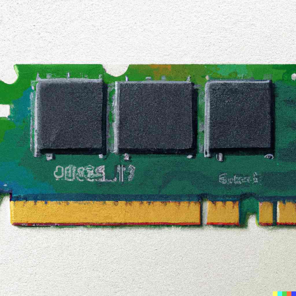
The advantage of a bad memory is that one enjoys several times the same good things for the first time.

― Friedrich Nietzsche

As a laptop or smartphone owner, you’re probably familiar with the amount of memory your device has. You are also likely aware that there are two types of memory that your device uses. For instance, let’s consider the latest MacBook Pro 13.

screenshot of the specs of a a macbook
Macbook Pro 13″ with M2 specs

The first line describes the RAM of each device, followed by the second line, which specifies the amount of secondary storage. Although both types of storage have distinct functions, they are equally essential for optimal device performance.

What are they

The primary function of secondary storage is to provide a permanent storage solution for your files, preventing data loss upon system restarts. Compared to RAM, which is designed to be fast and serve as the working memory for the CPU, this type of storage is cost-effective. For example, the M1 chip with its 16 cores can execute 11 trillion operations per second, requiring the RAM to be equally fast to avoid slowing down the CPU. RAM is costly and stores temporary data that is frequently cleared. In addition, RAM must be random-access, ensuring uniform memory access time.

The CPU can only access data stored in RAM, which means that anything a computer runs must be loaded into RAM first. Suppose you create a program that reads a text file with 10 numbers, adds them up, and writes the result to another file. In that case, your CPU will first direct secondary storage to copy the numbers to the RAM. The CPU will then execute the code to sum each number, updating the result in the RAM, and instruct secondary storage to write the outcome to a file.

A closer examination of RAM’s hardware implementation is required to gain a better understanding of how it works.

The RAM in your computer

Although there are various ways to implement a circuit that can achieve the same end result, for the purposes of this discussion, I will be using a basic DRAM (which is one way to implement RAM).

A quick detour

Before we go any further, we need to look at two components; the transistor and the capacitor.

the symbol for a transistor
The symbol for a transistor

The transistor is an electronic device that can be used as a switch or an amplifier. It has three terminals called Source, Gate, and Drain. When a current is applied to the Source terminal, it will only flow to the Drain terminal if a current is also applied to the Gate terminal. The Gate terminal acts as a control switch, determining when the current from the Source flows into the Drain. This property of the transistor allows it to be used in a wide range of electronic applications, from digital logic circuits to power amplifiers.

current flowing into the source of a transistor but not to drain
Current flows through the Source but does not make it to the drain since no current flows through Gate.
current flowing through bough gate and source resulting in current flowing to drain
Current makes it to the Drain since both Source and Gate have current flowing through it.

The second piece of circuitry would be the capacitor. A capacitor is a device capable of storing some amount of electric charge. You can think of it as a tiny water tower of electric charges. You can “recharge it” by passing a current through it and “discharge” that charge later. This is how a capacitor is represented.

symbol for a capacitor
Symbol to represent a capacitor

Memory Cell

Now, we can put the two of these circuits together to build a circuit that stores one bit of information. We’ll call this a memory cell.

memory cell constructed by putting together transistor and capacitor
The drain of the transistor is connected to one end of the capacitor. The other end of the capacitor is grounded. The Ground is a way in physics to represent 0 Voltage

A quick recap on some physics here: To understand how electricity flows in a circuit, it’s important to remember that current only flows when there is a difference in voltage between two points. This difference in voltage is often referred to as a voltage “potential.” Conventionally, current flows from the positive end of a circuit to the negative end. For example, in a 1.5V battery, the positive end is at a voltage of +1.5V, while the negative end is at a voltage of 0V which results in a current flowing from the positive end of the battery to the negative.

a sample circuit on flow of current
Conventional current flowing through a circuit.

Returning to the memory cell circuit, we now need to perform hardware operations on it. We will define the state where the capacitor has stored charges as “1”, and the state where the capacitor is drained or has no stored charges as “0”. These states will be used to represent the data stored in the memory cell. Let’s call these functions SET() and UNSET().

SET()

Suppose we have a hypothetical function that sets the memory cell to “1” by charging the capacitor. To do this, we need to apply a current by setting a higher voltage at both the Gate and the Source of the transistor. To do this, we set a voltage across both the Gate and the Source. The current, therefore, passes through to the drain and flows into the capacitor thereby charging the capacitor.

charging the memory cell

Cut off voltage at the Gate to cut off the current flow. This will result in the capacitor having stored some charge but being unable to discharge it back out since the gate is closed.

a charged memory cell

UNSET()

To unset the memory cell or drain the capacitor of its stored charges, we simply need to open the Gate of the transistor by setting a high voltage at the Gate and grounding the Source (setting it to 0V). This breaks the connection between the Source and the Drain, providing a path for the stored charges in the capacitor to flow out through the Source wire, effectively draining the capacitor. By doing so, we set the memory cell to “0”, which represents the absence of stored data in the cell.

draining a memory cell
Charges flow out of the capacitor on opening the gate.

Okay! So we are now covered in setting and unsetting the memory cell. We can extend the UNSET operation to perform a READ operation.

READ()

So during the UNSET operation, you allow the charges to flow back out through the Source wire by enabling the Gate and grounding the Source. Now say we had dedicated hardware plugged into the Source wire that was capable of detecting changes in voltage on this wire. So when the charges of the capacitor flow into the Source wire, there is a tiny difference in voltage across the Source wire which can be detected.

This is pretty much how a read operation takes place. The capacitor is allowed to temporarily discharge just a little bit so that the voltage difference can be sensed.

This does mean that you need a separate circuit to refill the charges lost during reads and this process is referred to as Memory Refresh you can read more about it here.

Now, it’s time to build ourselves some RAM!

Let’s construct our RAM

To construct our RAM, all we have to do is to arrange a whole lot of memory cells in a grid.

dram implementation by putting together memory cells in a grid
DRAM implementation

In practice, it’s not very useful to be able to read just one bit at a time. Modern computers define their own unit of memory known as a “word.” A word is a fixed-size block of memory that the computer can manipulate as a single unit. For instance, the M1 chip uses a 64-bit word size, which means that it deals with memory in blocks of 64 bits rather than individual bits.

By organizing memory into words, computers can read and write data much more efficiently. For example, when a computer reads a 64-bit word from memory, it can process 64 bits of data at once, which is much faster than reading each individual bit separately. This approach also helps to simplify the memory addressing and management process, making it easier for the computer to access and manipulate large amounts of data.

To understand how memory is organized in modern computer systems, we can take a look at the concept of word lines and bit lines. Word lines are a set of electrical wires that connect to each row of memory cells, while bit lines are another set of wires that connect to each column of memory cells. The number of word lines is determined by the amount of storage available in the chip, while the number of bit lines is typically the same as the word size.

For example, the 8086 processor uses 16-bit words, which means that each word has 16 bits. This means that there are 16-bit lines, one for each bit in the word, and the number of word lines depends on the total amount of memory available in the system.

Reading From RAM

So say you want to read the 3rd word in memory.

We kick things off by slightly charging up all the bit lines in our circuit with a small voltage. This keeps the current ready to flow at the Source but is unable to do so since the Gate is closed.

charging bit lines in dram
A small voltage is applied on all the bit lines.

Now, set a voltage across the 3rd-word line

charging word line to read in dram
A voltage is applied across the word line to be read. Note that the bit lines are still a little charged but an active voltage is no longer applied to them.

We’ve effectively opened the gate for all the transistors for word line 3. One of two things can happen at each bit line

  1. The capacitor it was connected to was charged. The capacitor’s potential is stronger than the mildly charged Source wire, therefore current flows from the capacitor into the bit line. (this is why we intentionally applied a lesser voltage on the bit lines). This flow of current into the source wire/bit line leads to a slight increase in the voltage at the bit line which can be detected as a 1.
  2. The capacitor it was connected to was empty. Now, the current from the bit line is able to flow into the capacitor. This loss of charges on the bit line leads to a slight reduction in voltage across the bit line which again can be detected as a 0.

After the read, to make up for the lost charges, the hardware that detected the voltage difference also re-writes into the capacitor that lost charges and drains the capacitor that had some charges flowing into it.

And there you have it, we’ve effectively built a miniature version of a RAM using a 1T1C (1 Transistor / 1 Capacitor) memory cell!

A Wrap for Part 1

The original plan was to write about how secondary storage works in the same blog post. But seems like we’ve covered quite a lot of new stuff already and anything new might just turn into an information overload. So let’s call it a day and continue the remaining of this blog in another post. If you’re looking for more interesting reads, check out how a computer actually manages to do math here.

The Flow Of Electricity and Math

robot doing math

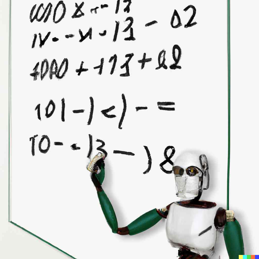
In the last post, we covered a little bit about what it means to be writing code (you can check it out here). That is, we briefly discussed what you and I see when writing code. But to a computer, the little python script we wrote really makes no sense. After all, it’s no different from any other text file you store on your computer.

If you’ve ever taken a class on anything related to computers in school, you’ve probably heard the phrase “a computer only understands 0s and 1s”. Although that statement is an over-simplification of what happens under the hood, there’s some truth to it. So in this post, let’s try to see what it really means for a computer to only understand either a 0 or a 1.

FYI, most of my images are generated by AI and have no real reason for being on my posts 🙂 Check out DALL-E tho

Let’s work our way up here. We start with logic gates. (I’ve skipped a few levels such as transistors. We can get into that in a different post).

So… Logic Gates?

Logic gates are little electrical circuits and as the name suggests implement a tiny bit of logic (duh).

An example logic gate

They’re made of transistors and essentially are little circuitry that manipulates the way electricity flows. Let’s take an example; the AND gate.

The AND Gate

The AND gate takes two input signals/wires and spits out its output on a single output wire.

The symbol for an AND gate

Here, you can see two different wires going into the AND gate, namely A and B. Each input can be in one of two states; either there’s electricity flowing through that wire or not; that is, it’s either a 1 or a 0. This is the origin of “computers understand 0s and 1s”.

The resulting wire represented by A·B can also only ever be two outputs (well… like all wires, there’s either electricity flowing through the wire or not; that is, 1 or 0). But for an AND gate, the result wire A·B is only ever 1 if BOTH A and B are 1 (that is, if and only if both A and B have electricity flowing through them, will the AND gate allow electricity out). That’s the “logic” part. How does the AND gate work? We’ll have to look into the transistors that make up the logic gate and to keep things simple, we’ll have to skip that part.

Anyways, the function of a gate can be represented in a tabular format popularly referred to as the Truth Table. Let’s take a look at what the truth table of an AND gate looks like.

AB A·B
000
010
100
111
The truth table for an AND gate. Only when A and B are 1, A·B is 1.

As you can see in the above table, only when A and B are both 1, the result is 1. In every other scenario, the result is a 0.

The OR Gate

Just like the AND gate, there are several logic gates that are of interest to us. Firstly, there is the OR gate whose output results in a 1 if EITHER A or B are a 1. The truth table would look as follows

AB A + B
000
011
101
111
The truth table for an OR gate. As long as either A or B are a 1, A + B is 1.

The XOR Gate

Then there’s the XOR (mutually exclusive OR) gate, whose result is a 1 if EITHER A or B have a 1 but not both. The truth table looks as follows.

AB A ⊕ B
000
011
101
110
The truth table for an XOR gate. As long as only one of A or B is 1, A ⊕ B is 1.

There are several other logic gates out there. Each is represented by a unique symbol assigned to it.

Alright! So now that we understand logic gates a little better, let’s go one step higher and make something meaningful out of these logic gates. Before we do that, I want to take a quick detour and explain binary numbers.

Binary numbers 101

In the decimal system, we use a base of 10. What that really means is, there are only 10 numbers (0 to 9). So, when you perform 9 + 1, you really have no other number left. So to solve this dilemma, what you end up doing is, you reset back to 0 and carry over the spillage to a new place resulting in 10. The 1 in the 10’s place basically indicates that the original number can be represented as 10 * 1 + 0. So taking a random number, 125, this is basically 10^2 * 1 + 10^1 * 2 + 10^0 * 5 (no surprises there I hope?).

Binary numbers follow all the same rules except using a base of 2. So instead of the flip-over happening at 9, it happens at 1. A binary number 1011 is nothing but 2^3 * 1 + 2^2 * 0 + 2^1 * 1 + 2^0*1 which equals the number 11. The rules for addition for example are the same too.

Adding the number 11 with the number 7 in binary. The rules for carry-over are the same. When you hit a number bigger than 2, carry it forward.

Our little adder circuit

Alright, so now, we’re going to challenge ourselves a little bit. Let’s construct a circuit that adds 1-bit numbers (a bit is a fancy way of saying a binary number) using the logic gates we’ve learned about.

Some quick binary math first

I like to start off in these situations by constructing the truth table first and then building the circuit accordingly. Let’s see if we can piece this together. In all the truth tables so far, we’ve only had a single output. But for my adder, let’s have two separate outputs, Sum and Carry-Over.

What just happened here?

Carry-Over will represent the part that gets carried over during addition (if any). Sum will represent the part that we write down. Don’t worry if this didn’t make any sense. This part should help clarify it.

Okay…? How did I do this? Let’s walk through this table a little bit. So since I expect this bit to be a little confusing, I’ve broken down each case one by one.

I’d recommend going over this image and comparing it with the truth table above to make sure it checks out

We’ve defined Sum to be what we write down (completely ignoring the carry-over). Carry-Over is the part that gets actually carried over. If you look at Case 4 specifically, the sum of 1 and 1 is 10 in binary. The Sum part of that would be the 0 we actually write down and output the carry over in its own output.

So now, I hope you’re convinced that the truth table for our addition checks out. Based on the truth table, let’s try to reverse engineer the circuit we would require to produce the same output as our truth table.

Time to build the circuit

First, let’s figure out how we’d generate the Sum column given inputs A and B. If you refer back to the truth table of the XOR gate (don’t be lazy. scroll back up and check the truth table for the XOR gate), you’d see that the Sum column is nothing but the XOR of A and B.

Secondly, if you look at the Carry column in the truth table, you’ll see that the Carry column is nothing but the AND gate’s truth table with respect to inputs A and B.

So there we go! Let’s see what the circuit would look like for a 1-bit adder. The circuit would take two inputs, and spit out two outputs, which would be the Carry and the Sum.

This circuit is what we refer to as a “half adder”. A similar circuit can be generated for taking 3 inputs which is referred to as a full-adder circuit.

Putting all of this together

From here, we can work our way further. The above circuit adds two 1-bit numbers. If you want to add two 2-bit numbers, you chain similar circuits together (you’d also use the Carry as an input) until you have an adder for a 2-bit number.

Remember our function add_numbers in the last post? We defined a function and invoked it later by calling its name along with the arguments as its input. A modern processor does something similar. The processor in your computer comes with an “instruction set” which is a set of basic instructions that the processor is able to perform. (Here is an example set of instructions that the x86 family of microprocessors use). When you write any piece of code, you run it by another software to convert it from the human-readable version into a series of instructions that your computer can actually understand (instructions that are specified in the instruction set).

For example, the x86 instruction set supports the ADD instruction which adds two 64-bit numbers. (Just take the 1-bit adder circuit, chain it up a few times and make a 64-bit adder). When your compiled code contains an ADD instruction, your computer takes the two binary numbers and passes electricity through just the wires that are specified by the input numbers. The circuit logic will “do the addition” by essentially looking at which output wires contain electricity.

And that’s a wrap!

We started from a basic logic gate, something that took two 1-bit binary numbers and implemented some bare minimal logic. Out of that, we built an adder which combined some of these logic gates to do something more. We then chained several of these 1-bit adders to get a 64-bit adder. And now, each time your computer runs any program, electricity flows through this circuit to do your computation.

A Brief Introduction To Programming

corgi writing a program

If I’m being candid, there is already a whole bunch of content out there on the subject of programming. (If you want to get started on a full-blown course learning how to code in Python, for example, I’d start with FreeCodeCamp)

However, if somebody was trying to explain to me how the engine of a car worked, it would be a very confusing lesson if I hadn’t the slightest clue on how to drive. Someone who can drive may not necessarily understand what happens when you “hit the gas” but is at least a little better equipped to understand how things work. So let’s go for a drive!

a hackerman who is visibly frustrated as his unit tests fail for no apparent reason
Me busy at work. True story

Programming, at its core, is all about data manipulation. You give your code an input, it performs the set of instructions you’ve asked it to on that input and it gives you an output. The input can come in a lot of different forms; numbers, text, images, and so on. They can also come from a variety of sources; user-provided input, computer-generated input, over a network, from a database, (you get the point…). Once you have this input, you can write “code” which is basically a set of instructions telling your computer how to manipulate this data to get a useful output out of it.

Let’s look at our first ever python script!

def add_numbers(num1, num2):
	return num1 + num2

first_number = int(input("First number: "))
second_number = int(input("Second number: "))
result = add_numbers(first_number, second_number)
print(result)

Let’s run this piece of code now. I’ve saved this file as test.py

~ python3 test.py 
First number: 5
Second number: 10
15

Underwhelming? Probably. But let’s take a better look at what this snippet is really doing. (Okay now, I might butcher some of the lingoes for the sake of clarity. So I apologize to my fellow nerds ahead of time).

Remember how I said that all a piece of “code” does is take an input, do something with it, and return an output? You’d be able to see that pattern all over this script that we just wrote. In programming, something is called “a function” if you can invoke it by its name (bear with me here). If you see Line #1, I’ve defined a new kind of function called add_numbers which takes two inputs num1 and num2. And what does this function do? That part is defined in Line #2. The function is expected to give back num1 + num2. That’s what the return keyword is for. It asks the function to compute num1 + num2 and give back the result to whoever invoked the function. The indentation in Line #2 (the blank space before the return keyword) indicates that Line #2 is part of the function body and not a part of our overall snippet. (You’ll see that Line #4 for example does not have any blank space before it. This is how python knows what part of the code belongs in the function body and where the function body ends). Only at Line #6 is when I actually go ahead and invoke the function by its name add_numbers along with the inputs this function takes which are comma-separated inside the parentheses add_numbers(first_number, second_number).

Just like how we defined our own functions, python comes with a set of pre-packaged functions that we can use. The act of taking input from the user is a pretty commonly used functionality in most programs and therefore, you’d see the input function on Line #4. I did not define a input function. I knew Python had a built-in function (Link to docs) for this. And as the doc mentions, you can pass the prompt to be displayed as part of the input collection process which I specified as "First number: ". Similarly, the int function on Line #4. I knew that the input function outputted a string but I wanted an integer since I was looking to add those numbers. Therefore, I passed the output of the input function as the input to the int function so that the int function could give me the integer equivalent. The same line could have been broken down as follows:

string_number = input("First number: ")
first_number = int(string_number)

Okay, this is the last part of the code I’ll talk about. Do you see the left-hand side of any of these lines? string_number = input("First number: "). What we’re instructing python to do is, compute the input function with the input "First number: " and store its output in a variable named string_number. A variable can be thought of as a box. The output of the input function is stored in a box named string_number which can now be passed along to other functions such as int as input.

Okay phew, that was quite a bit. But on the bright side, we’re now officially done looking at code snippets! For now…

Now, instead of looking at “code” as a black box, we can start thinking of it as a collection of “functions” strung together.

a tree format of the same code. functions are connected to each other via lines representing the flow of data
The same program with the flow of data visualised as a “tree”.

Alright. So far, we’ve seen that any code can basically be represented as a “chain of functions”; much like an assembly line in a factory. Data flows in, are acted on by functions and the result of this becomes the input of other functions down the line. But to be completely honest with you… this is a human representation of code. This isn’t what my computer saw when I ran python test.py. Or atleast, this isn’t the complete picture. I’ll save that part for another blog post.

Hello World!

astronaut waving

I’m not gonna lie… Writing this first sentence was surprisingly challenging. I ran through a million different scenarios on how I’d begin my first blog post. Should I sound formal or would it make more sense for this post to sound more like an informal chat with me? If you’ve ever played any of the Pokemon games on Nintendo and took forever to settle on an in-game name for your character, you’d probably understand my dilemma right now. (FYI, Emerald was my favorite. Still wish I was able to catch myself a Feebas in that itsy-bitsy lake on Route 119)

But anyways, enough for that. My name is Akshay Pai. I currently work as a Software Engineer at Google. I’d consider myself a nerd in every sense of the word. I enjoy binging on science-based content on Youtube (I’m looking at you Kurzgesagt 🫦). I love to read fantasy fiction (although to be fair to me, I do read other genres too). And if you aren’t convinced of my nerdism yet, you should know that I’m up to date on One Piece (I’ll give it a few minutes for that to sink in).

Now more importantly, why the blog you ask? Teaching people about programming and CS is something that has always been super close to my heart. To be able to take things apart and look at how things work under the hood is absolutely magical if you ask me. This blog is my first step in that direction. P.S: I am by no means a great writer (maybe this exercise will help me get better? but that’s really not the intent of this blog), but I do hope that this attempt to demystify Computer Science is helpful to somebody 🙂