

This is the first part of a series of posts in an attempt to piece together how your computer really runs your code. The topic by itself could have an entire book dedicated to it, but I’m going to see if we can cover the essentials without delving too much into the nitty-gritty details (after all, these posts are intended to be beginner friendly). A quick note before we get started, I am by no means an authority on the subject. If something seems inaccurate, please do let me know.
A quick recap on computers
Every computer comes with a series of hardware components. Let’s take a look at a Raspberry Pi 4 – a miniature computer.
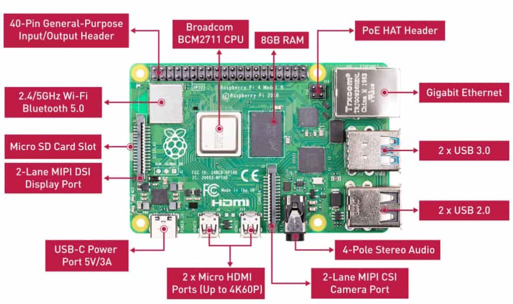
There’s quite a bit going on in this image, but what we’re interested in at the moment is the Broadcom BCM2711 CPU and the 8 GB RAM chips. Two of my previous posts briefly cover the workings of both of these (CPU, RAM). (There was supposed to be a part 2 for some of these topics but well… life is short and so is my attention span).
RAM
In a nutshell, the RAM can be visualized as a linear sequence of bytes that can be read or written to. Each byte in the RAM has a reference number we call “address”.
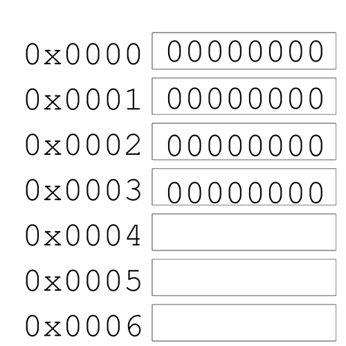
For example, the memory address 0x0000 (in hexadecimal) stores 1 byte (8 bits) of information 00000000. If you wanted to read the 285th byte in your RAM, you would want to access the memory location 0x011d (285 in the decimal system).
CPU
The CPU supports several basic operations your code could use which are defined by the manufacturer of the chip. This chip supports the ARM instruction set. The instruction set of a chip supports a fixed set of predefined operations such as ADD; which adds two numbers, or the LD/ST; which loads / stores data to a memory location (the full list of operations supported can be found online).
Your CPU doesn’t deal with individual bytes. A single byte is nowhere close to being large enough to store anything meaningful. Therefore, your CPU defines a “word”, which is the number of bytes that it typically works with at a time. This is what we mean by a “64-bit” computer. Your computer defines the word size to be “64 bits”. Or that is, it’s capable of working with 64 bits / 8 bytes of data at a time.
Apart from the memory in the RAM, a CPU comes with registers that are extremely high-speed memory locations that the CPU can use. Think of registers as the CPU (core)’s personal fanny pack while the RAM as a suitcase that it shares with the other cores. All the stuff that a core requires at any given moment is typically stored in the fanny pack. It’s easy to access but has limited storage.
A CPU comes with anywhere from 16 – 30 registers that it can use and each register is the size of the word, 64 bits for a 64-bit CPU. How are these registers used? Say you ask your computer to add two numbers, your CPU loads the two numbers from the RAM into registers, runs the ADD operation on the two registers, and stores the result back into the RAM (not always the case but it’s typical).
All of this should be a lot clearer when we see some examples in action. For now, all I want you to remember is the following:
- A CPU (core) comes with a set of registers which are high speed memory locations for the CPU to read and write to. A CPU also has access to the RAM.
- Any operations your CPU performs, has to either be performed on a register or in the RAM. If you want your code to modify a text file, it (or at least the part of it that you need to work with) needs to be loaded first into the RAM.
The End Goal
So, where are we going with all this? Essentially, whatever code you intend to run, needs to first be converted into something your CPU understands. What this means, is that each instruction in your Python / Java / C++ code needs to be translated into one or more instructions defined in the instruction set of your CPU.
There are several different approaches to go about this translation each of which have their own pros and cons.
Compilers
Languages like C / C++ take this route. Compilers convert your code into a low level language compatible with your computer’s instruction set. We call this converted code, assembly code. So each time you want to run your code, you “run” the assembly translation of your code. The translation to your assembly code is a one-time process (unless of course, you make changes to your code, you need to retranslate).
The advantage of this approach is that the compiler has translated your code into something that is native to your computer. So your computer has a fairly easy time when actually running your code.
But what happens if you want to run your code in a different system that runs a different architecture? The assembly code you generated was native to your computer and there’s a chance it might not work on my computer (if my computer runs a different operating system or has a different instruction set). Therefore, to run your code, I would need a separate compiler that knows how to translate your code to something my computer understands.
The Bytecode Approach
The downside in the previous approach was that the assembly we converted our code to was machine dependent. And the bytecode approach addresses just that. Here, we translate code to something that looks like the assembly we would have seen in the first approach except that this assembly is machine independent; which we call bytecode. Your code did get translated to something low level but it’s not something our computer understands (since after all, the only thing your computer can run is something its instruction set can understand). So… how do we run this on our computer…?

To actually run this bytecode, you need to have a separate piece of software running in your computer that is specialized at running your bytecode. We call this a “virtual machine” as this software mimics a computer whose instruction set is the same as that in your bytecode. This is a separate topic by itself so we’ll stop here for now. The key takeaway is that the advantage of bytecode is that it is independent of your computer hardware. The same bytecode that was built on your computer can be run on a different computer (as long as this different computer has a virtual machine installed that is able to run this bytecode).
Java typically takes this route.
Interpreters
This is the lazy way out (not necessarily a bad thing). The interpreter reads a line of your high level code, figures out how to translate this to something your computer can understand and runs this line before moving on to the next line. Notice how unlike the previous approaches, the interpreter translates AND runs your code in the same pass. In the previous approaches, you had your code translated to an intermediate low-level code (assembly / bytecode). Each time you want to run your code, you just need to run the low-level code directly as the translation has already been done. There is no need for retranslation each time you want to run your code.
Whereas in an interpreter, each time you want to run your code, the translation phase is redone.
This makes interpreted implementations of a language slower but it gives some added flexibility which we can explore in a separate post.
Wrapping it up
So far, we’ve covered the need to translate your code to something your computer can run and three approaches that are typically taken to get there.
Most questions however still remain unanswered. How does a compiler translate your code to something my computer understands? How does your code interact with various devices that your computer comes with (such as your monitor or WiFi) to make something useful happen? What does this assembly code actually look like and how does it actually run in your computer?
We’re still missing a quite a bit of context but I think we should be ready to see some basic examples. In the next post, we’ll see some of this in action on a 64 bit AMD computer that runs Linux.